Neural ODEs with stochastic vector field mixtures
It was recently shown that neural ordinary differential equation models cannot solve fundamental and seemingly straightforward tasks even with high-capacity vector field representations. This paper introduces two other fundamental tasks to the set that baseline methods cannot solve, and proposes mixtures of stochastic vector fields as a model class that is capable of solving these essential problems. Dynamic vector field selection is of critical importance for our model, and our approach is to propagate component uncertainty over the integration interval with a technique based on forward filtering. We also formalise several loss functions that encourage desirable properties on the trajectory paths, and of particular interest are those that directly encourage fewer expected function evaluations. Experimentally, we demonstrate that our model class is capable of capturing the natural dynamics of human behaviour; a notoriously volatile application area. Baseline approaches cannot adequately model this problem.
This blog post relates to some recent work of mine (Twomey et al., 2019) on neural ordinary differential equations. While the work is under review at the moment this post is going to introduce a high-level summary of the main ideas of the paper, and all of the details can be found in the PDF (link can be found at bottom of page).
Introduction
The figure below shows a classification problem with two intersecting ‘moons.’ This is a fairly well-known dataset whose topology is relatively simple but the task is still not linearly separable, or in other words you cannot draw a straight line through the figure such that all blue points lie to one side of the line and all orange points lie on the other side.
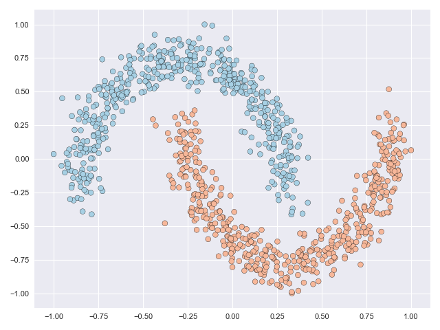
But what if we are allowed to subject the data to some kind of transformation before drawing the line? In this post I’ll illustrate how neural ordinary differential equations (NODEs) offer a flexible framework that can make the problem above linearly separable (and more!) without relying on, say, dual representations. We introduce some new ideas to the NODE setting in the paper linked to below and our contributions boil down to two essential questions:
- How can we make the transformations simple?
- How can we make the transformations flexible?
You may (quite reasonably) think that if you optimise one of these that you will surely have to compromise on the other… but it turns out that with the approach we propose this isn’t the case at all, and you can enjoy the best of both worlds!
Example
The NODE framework is very robust and can subject data to complex and non-linear mappings. The characterisation and complexity of these mappings is optimised during the learning process. Without going into the details (these can be found in the paper) the figure below animates the NODE solution of the moons dataset with some constraints that we introduce in the paper. The main takeaway from this image is that even though the original data is not linearly separable, the final transformation is.

The transformations shown above depict the paths travelled by the particles (datapoints) through a vector field over an integration interval. The vector field can be thought of as a force that acts on the particles, and the objective of NODE models is how parametric vector field producing functions can be learnt so that they do something useful.
Notation
Vector fields are defined as follows in the NODE paradigm
\[~~~~~ \nabla \mathbf{h}(t_i) = f(\mathbf{h}(t_i), t_i; \boldsymbol{\theta})\]where \(\mathbf{h}(t_i)\in\mathbb{R}^D\) is a hidden state at depth \(t_i\) (base state \(\mathbf{h}(t_0) \triangleq \mathbf{x}\), maximal depth \(t_T\)), \(f\) is a neural network of arbitrary architecture and \(\boldsymbol{\theta}\) are its parameters. Subsequent hidden states are derived by taking small steps from \(\mathbf{h}(t_i)\) in the direction of the vector field, i.e. \(\mathbf{h}(t_{i+1}) = \mathbf{h}(t_i) + \delta_{t_i} \nabla \mathbf{h}(t_i)\), and the step size \(\delta_{t_i}\) is often selected automatically by an ODE solver. The solution of this initial value problem is obtained by repeatedly taking these steps until the output state \(\mathbf{h}(t_T)\) is reached, and these outputs may undergo a final transformation, eg through a softmax layer in classification tasks. The optimisation objective is to adjust the dynamics of the ODE through \(\boldsymbol{\theta}\) to maximise the data likelihood.
What makes transformations complex?
Several things contribute to complex paths, and complex paths can not only jepordise model fit but will also require more time (evaluations) to determine solutions. Two complexity-inducing aspects that we penalise in our models are
- Paths that span long distances
- Paths that encounter curvature
The two animations below illustrate what complex transformations look like on the moons and circles datasets. In particular with the moons dataset, the data can be seen to do an unnecessary rotation before the classes eventually separate. But the feature range of both datasets is scaled significantly due to the transformation. The inner circle has to ‘break through’ the outer circle in the circles example, and this process requires many function evaluations.

How to make simple transformations
It turns out that we can fairly straightforwardly penalise long and curved paths. A loss on the path length can be formulated as follows:
\[~~~~~ \mathcal{L}_{\text{TLoss}} = \frac{1}{T} \sum_{i=1}^T\| \mathbf{h}(t_{i}) - \mathbf{h}(t_{i-1}) \|_2^2\]which is simply the sum of the Euclidean distance between successive evaluation points, i.e. the total transportation distance.
It’s reasonably easy to see that high variance vector fields are indicative of a turbulent trajectory while low variance vector fields are suggestive of a straight trajectory that is simpler to solve. A loss on the curvature of vector fields will then encourage straight vector fields, and this loss is formulated based on vector field variance as follows:
\[~~~~~ \mathcal{L}_{\text{VLoss}} = \frac{1}{T}\sum_{t=1}^T \left\| \nabla\mathbf{h}(t_i) - \mathbb{E}\left[\nabla \mathbf{h}(t)\right] \right\|^2_2\]where \(\mathbb{E}\left[ \nabla \mathbf{h}(t) \right]\) is the expectated vector field over the path.
So, by integrating these two penalties into the problem we hope to achieve transformations that have a small total distance traversed and whose transformations are mostly linear. The balance between these path-based losses and the classification objective will ultimately define how simple the actual trajectories are.
Let’s see how successful these methods are in simplifying the solution paths from those shown above. In the animations below, we can see that in the moons dataset a very straightforward transformation was achieved, and only a small fraction of the datapoints actually move. In the circles dataset, the task is much more complex but the task is solved without requiring the inner circle to ‘break’ through the outer circle. Notice as well that the scale of the figure axes does not increase.

How to make flexible transformations
The key to introducing flexibility to these models is to posit a mixture distribution over a set of vector fields. Instances are assigned to a particular component (vector field) based on, for example, their starting location in space, and instance trajectories are influenced only by that vector field. The figure below illustrates this. The curved line is the boundary for assigning component membership: everything above this line is assigned to one component while everything below this line is assigned to the other. The transparency of the transported datapoints indicates the probability with which they were assigned to a component. The characteristics of component membership are determined automatically by the modelling framework.
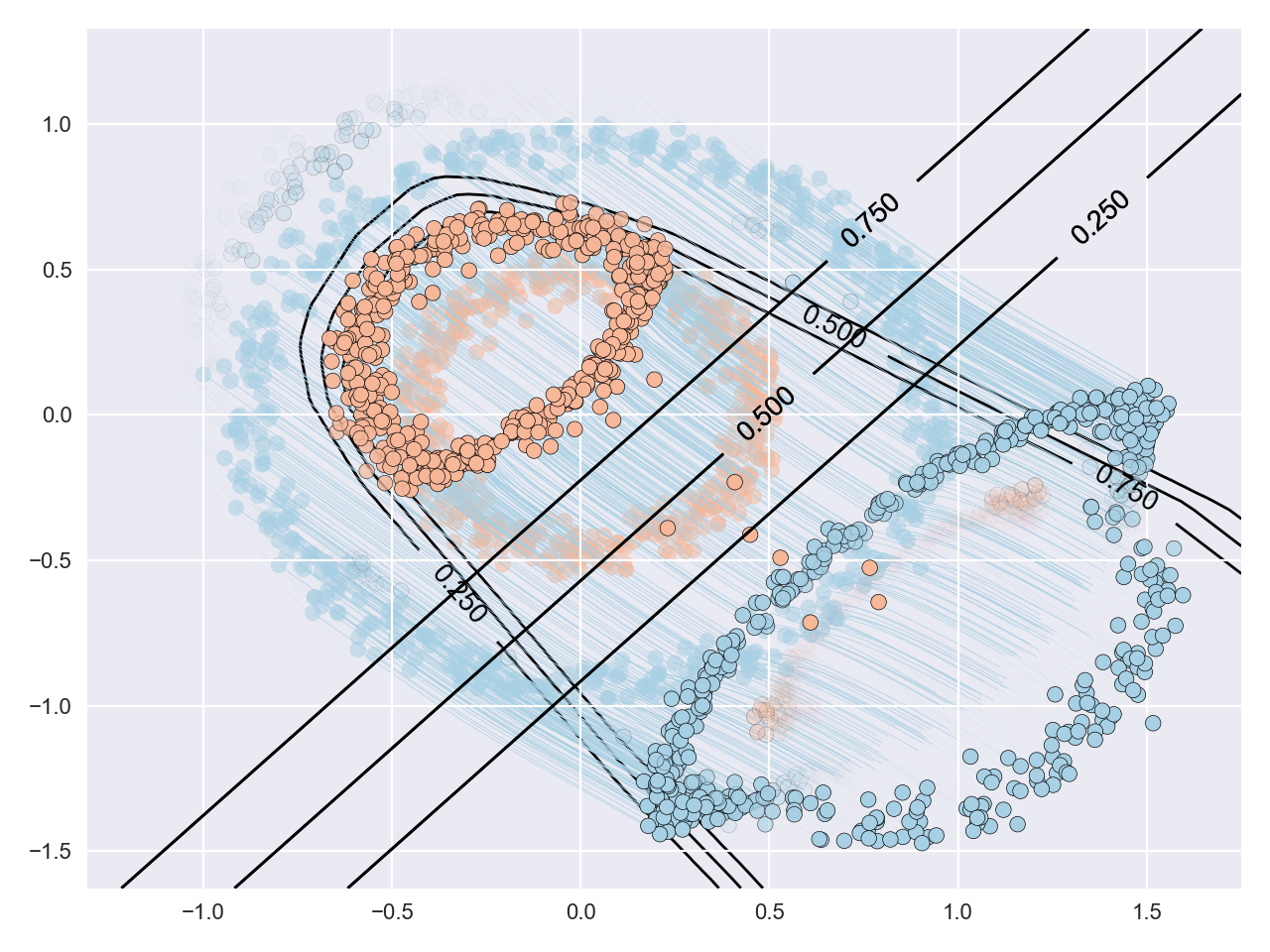
The datapoints assigned to the respective components travel without being influenced by other vector fields. In a sense, this allows datapoints in different components to ‘pass through’ each other. This is illustrated in the animation below where we can see the orange and blue datapoints pass over one another in opposite directions in the second frame. Of particular note is the speed at which this solution is achieved. All of the animated GIFs in this page have the same frame rate, and since this animation is approximately 2-3 times faster than the others shown the solution was given with 2-3 times fewer evaluation positions.

Aside from the uncertainty introduced to our model with the mixture distribution, our paper also introduces uncertainty on the vector fields themselves. Our vector fields are probabilistic and (roughly) follow a Gaussian distribution. The effect of this is to produce a one-to-many mapping from the original datapoint to a set of possible endpoints. Our experiments show that this seems to act as a regulariser on the solutions (since in training a wider set of endpoints have been explored) but vector field uncertainty is an essential component for enabling forecasting in human behaviour modelling applications, and these are introduced below.
Human behaviour modelling
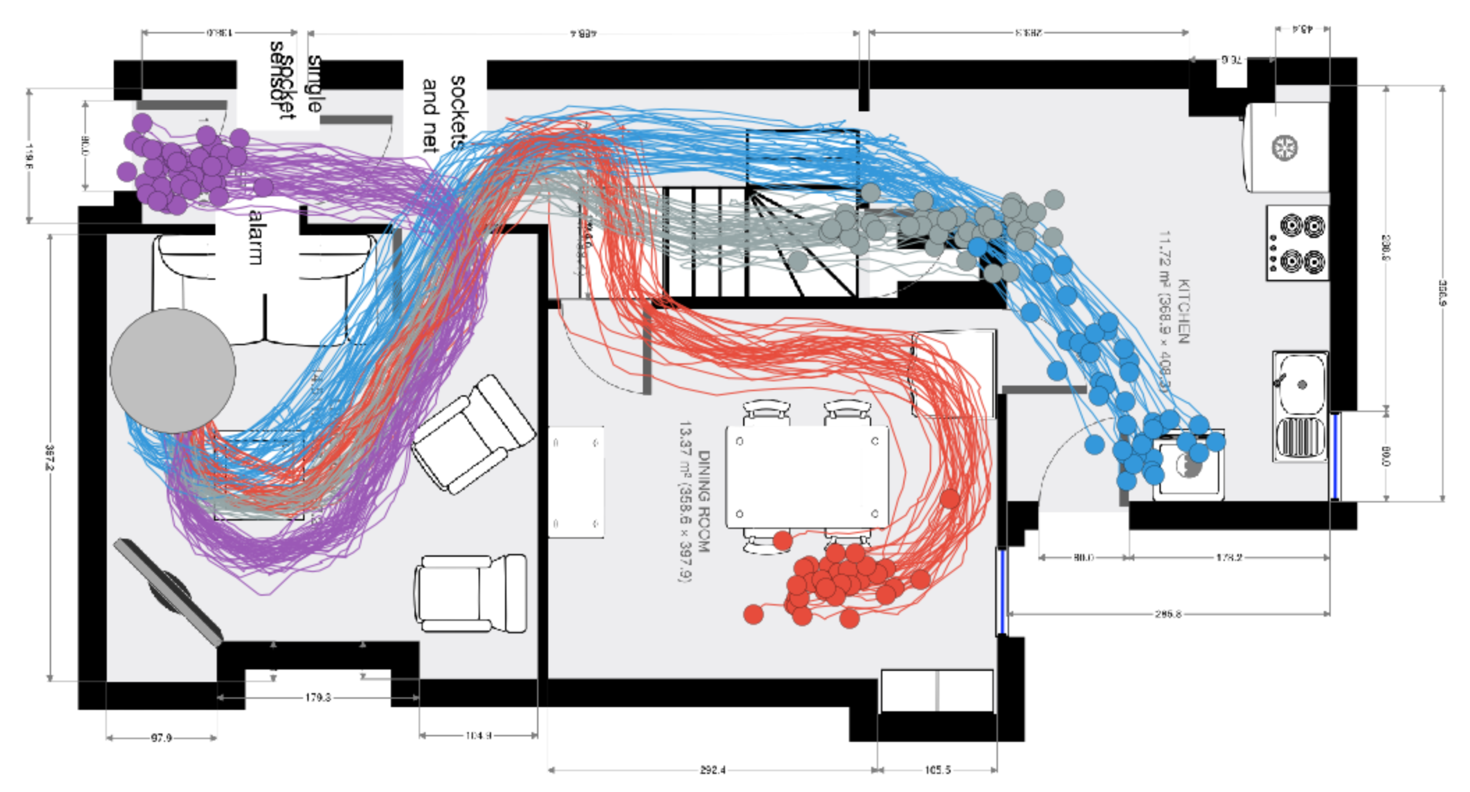
In behavioural forecasting we are interested in predicting the future location and trajectory of a person given knowledge of their original starting position. Our models (called stochastic vector field mixtures (SVFMs)) utility in delivering these forecasts is demonstrated with a dataset captured in a residential environment. A volunteer was recorded with a LIDAR data collection unit and the resulting point-cloud was processed with SLAM techniques to produce location data on relative reference frame. This dataset effectively captures characteristic behaviour in a home setting, with a particular focus on the types of behaviour following a departure from the living room.
SVFM models are learnt from this dataset. The main difference between this modelling problem and the previous classification problems is that in forecasting every single intermediate evaluation point is and contributes to the loss (and not just the final point, like in classification). In other words, you cannot go from the living room to the kitchen without first traversing through the downstairs hallway.
SVFM models can be samplled since they are probabilistic. A sample in this case depicts a path deemed to be ‘typical’ by the SVFM model. Approximately 20 sample paths are are shown in the image below. Notice that while the broad direction of the paths is shared, every sample follows a slightly different trajectory due to the uncertainty on the vector field.
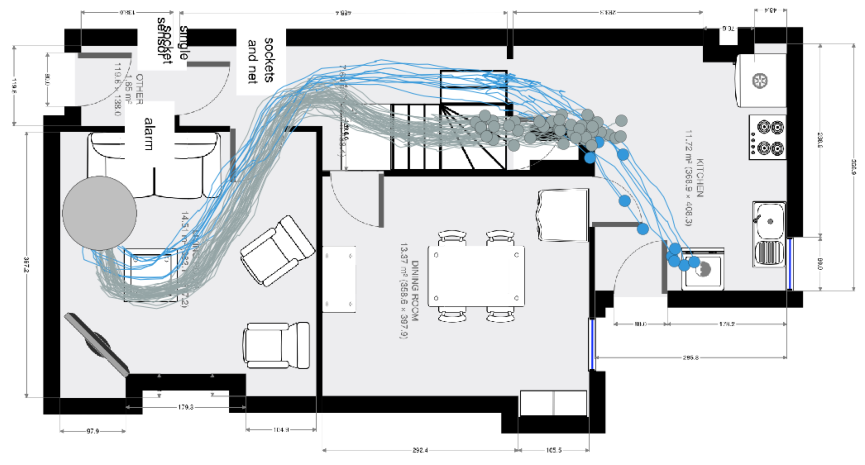
We also showed that these models can contextualise predictions based on the time of day. The image below shows the forecasted endpoints very late at night and a clear preference for climbing the stairs (i.e. to go to a bedroom) is shown.
Take-away messages
I hope this has given a flavour for some of the capabilities of NODE and NODE-like models (such as SVFM that we propose in the paper below). While I think the classification tasks are very informative for understanding and learning about these model classes (and for motivating useful regularisers), I also believe that the forecasting example delivers a more complete illustration of the model’s capability. This is because neither NODE models (nor a variant called Augmented NODEs) are capable of solving the behavioural forecasting problem. SVFM paths are richer (both by the mixture distribution and the uncertainty on the vector fields) and thus may model a broader set of problems, including behavioural forecasting.