Taking the Fourier transform of your cat
There are a few YouTube channels that I watch fairly regularly that have recently been making some truly beautiful visualisations of the Fourier transform. The visualisations really were beautiful (I'll link to them in the text) not only aesthetically but also in how they intuitively show what the Fourier transform works and what it achieves. I was inspired to try to replicate the visualisation procedure and the code inside this post is a python implementation of the method. The approach itself in truth isn't terribly complicated, but I find the outcome hypnotic!
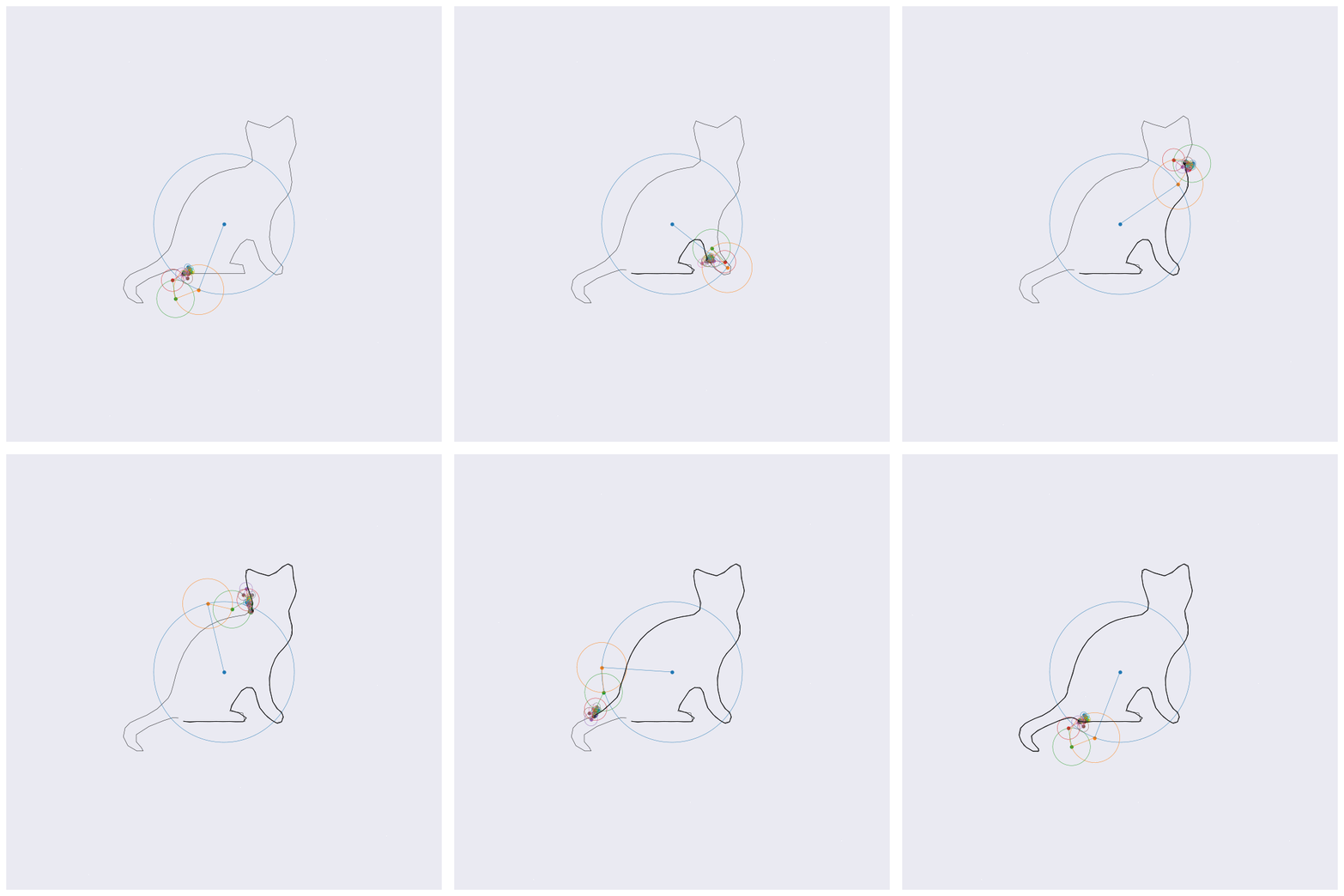
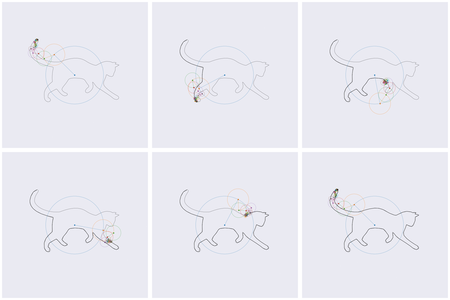
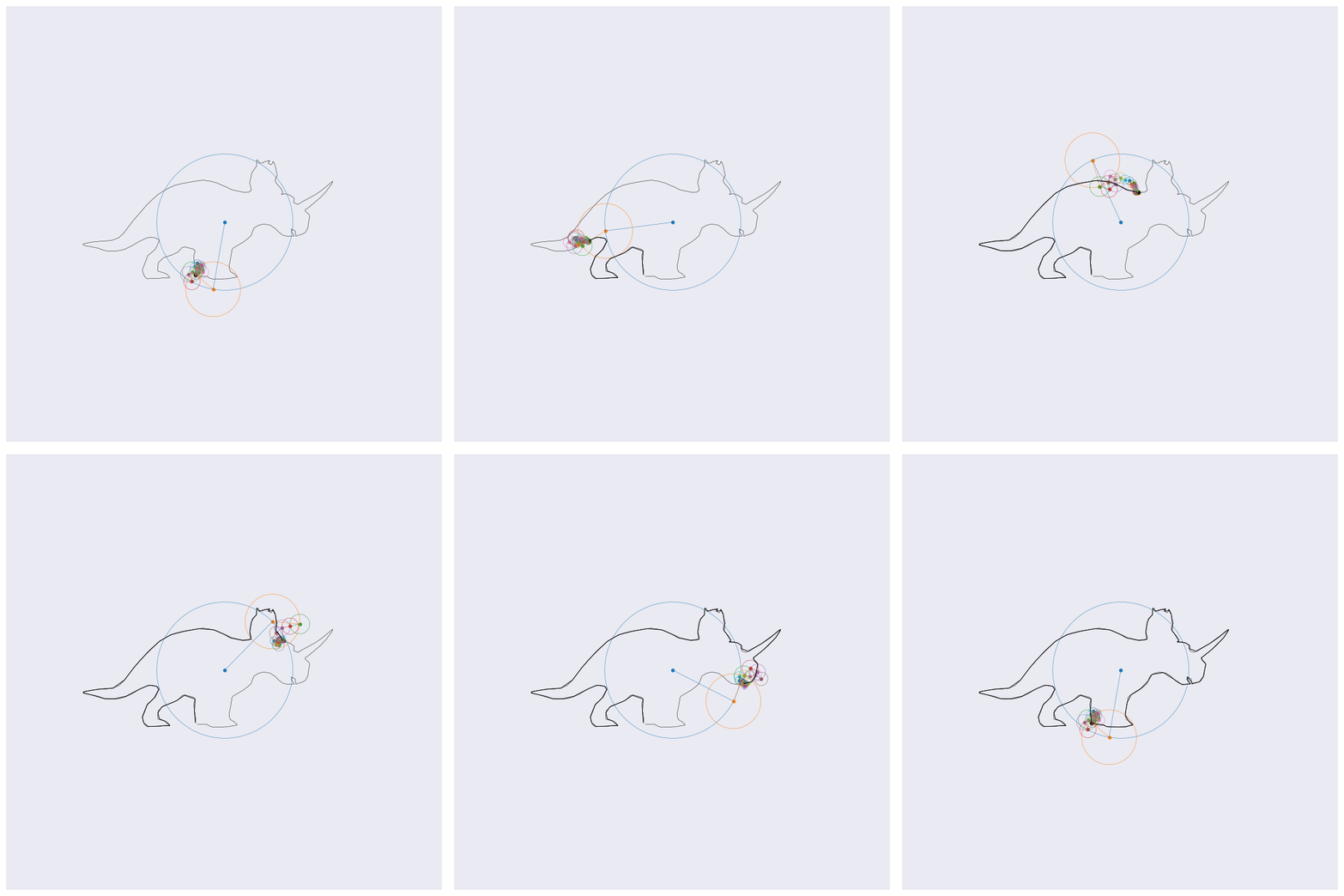
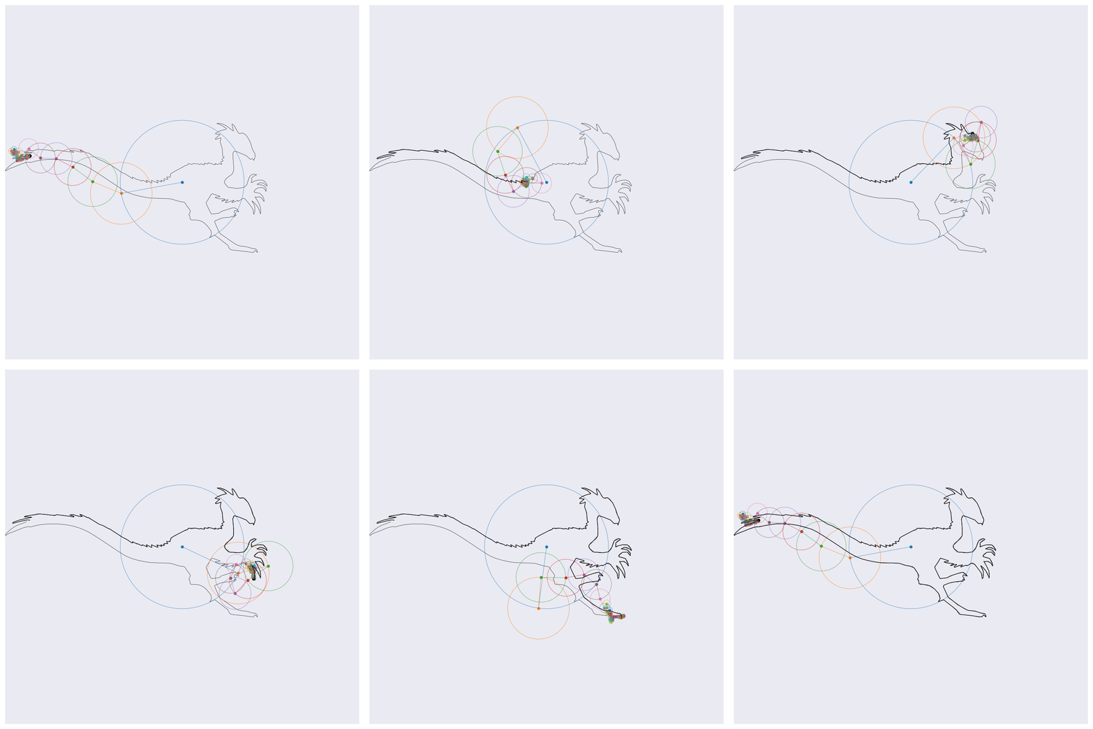
Before getting into the coding, here are four example outputs of the code that I’ll be generating:
I’m not going to try and explain how this works in any great detail since there are two excellent videos that deal with these ideas here and here (Grant Sanderson’s YouTube channel has been teasing about a video on this exact topic for weeks and I’m very much looking forward to this!). After watching these videos I really wanted to play with the main idea here. Unfortunately the code they had was in Mathematica which I don’t have installed on my computer (and anyway I haven’t used for over a decade) so I thought it would be a fun exercise to implement this in Python. The code I produced as well as some example SVG images for the cats and dinosaurs above can be found here.
If you know about Fourier transforms, not much here should be too surprising. The main point to take is that the Fourier transform decomposes signals into a weighted sum of complex exponentials (circles, essentially). By stacking these on top of one another and by rotating through them according to their individual rates, the orignal function will be perfectly reconstructed. This is the essential idea behind the images shown above, except for computational efficiency I’m approximating the functions with 99% resolution (loosely speaking) which loses some of the sharp edges.
The code below calculates everything needed to begin the GIF generation process. Remarkably, the first line np.fft.fft(f) does all of the computation that is needed to produce the images above. The rest of the code is just scaffolding for loading data and producing the animation.
def transform(f, threshold=0.99):
    # Calculate the FFT of the data
    F    = np.fft.fft(f) / f.size
    freq = np.fft.fftfreq(F.size, 1 / F.size)
    M = np.abs(F)

    # Select the number of components
    inds = np.argsort(-M)
    M_norm = M / M.sum()
    M_norm = np.cumsum(M_norm[inds])
    N = (M_norm < threshold).sum() + 1

    print(f'Evaluating with {N - 1} components')

    # Get the indexes of the top freqencies and slice these
    top_inds = (inds[:N])
    top_inds = top_inds[top_inds != 0]

    F_sel = F[top_inds]
    M_sel = M[top_inds]
    freq_sel = freq[top_inds]

    return N, F[0], F_sel, M_sel, freq_sel
The snippet below draws the stacked circles on top of one another for a given timepoint t. The function plot_circle is found here and the segment np.exp(1j * f_i * t) does the incremental rotations around the circle.
points = []

# ...

for ti, t in enumerate(np.linspace(0, 2 * np.pi, 100)):
    v = F_0
    pl.clf()
    pl.plot(f.real, f.imag, 'k', lw=0.5)
    for ci, (F_i, M_i, f_i) in enumerate(zip(F_sel, M_sel, freq_sel)):
        r_i = F_i * np.exp(1j * f_i * t)
        pl.scatter([v.real], [v.imag], c=cmap[ci], lw=0.25)
        plot_circle(v, M_i, t, r_i, colour=cmap[ci])
        v += r_i
    points.append(v)
    pl.scatter([v.real], [v.imag], c='k')
    pp = np.asarray(points)
    pl.plot(pp.real, pp.imag, 'k', lw=1)
I wrapped all of this up in a python file that can be called from the command line to produce these animations with simple SVG images as inputs here. If you’re trying out new SVG files you may need to make some image-specific adjustments in the load_svg function like I did here.
python make_animation.py --precision 0.99 cat1.gif
I think these animations are entirely hypnotic to look at and the rotational behaviour is very beautiful. I find it remarkable given this how easy it is to produce these images especially since I have understood and used Fourier transforms in dozens of projects over the past decade and never had this in mind when doing so. Amazing stuff!


